Matrices
Objective
Get exposed to matrices, basic matrix operations, and what it means to multiply a vector and a matrix.
Matrix Notation
Sometimes in software, we need to use an array of arrays (or a two-dimensional array, where the inner arrays are all the same length). In C-like languages, we might create one with something like this:
int[][] matrix = new int[3][];
for(int i = 0; i < matrix.Length; i++)
{
    matrix[i] = new int[2];
}
Or, if the language supports explicit multi-dimensional syntax, something like this:
int[,] matrix = new int[3,2];
Both of these would create two-dimensional arrays with 3 elements in the first dimension, and 2 in the second. Similar to how vectors are the general math version of arrays, the math version of a two-dimensional array is called a matrix. Matrices have the same syntax as vectors (number wrapped in square brackets). The first dimension is represented by the rows of the matrix, and the second is represented by the columns. Here is an example of a 3x2 matrix:
When referring to a matrix in your code comments, one common convention is to write each row out with commas, then separate the rows with semicolons. The matrix above would be written like this:
// This matrix will be [1, 2; 3, 4; 5, 6]
As you might expect, matrices essentially act the same way as vectors during arithmetic operations. In fact, a vector is really just a matrix where one of the dimensions is 1.
Matrices are represented by regular old algebraic variables, though they're usually capitalized to distinguish them from constant values or vectors. Elements of a matrix \(A\) are usually referenced with two subscript indices, where the 1st is the row and the 2nd is the column, like this:
Math Properties
Addition
Adding two matrices together is the same as adding two vectors. The matrices must be of the same size. Just add each element to its partner:
Scalar Multiplication
To multiply a matrix by a constant factor, just multiply each element by it.
Matrix-Vector Multiplication
One of the most common operations in quantum computing is multiplying a matrix with a vector. To multiply a matrix and a vector, there is one precondition: the length of the vector must be the same as the width of the matrix (the number of columns it has).
To do the multiplication, flip the vector sideways (so it becomes a row vector) and calculate the dot product of each row of the matrix and the vector. The result will be put into a new column vector, which has the same height (number of rows) as the matrix:
It can help to think of the matrix above as representing a function that takes in the vector \(\begin{bmatrix} x_0 & x_1 \end{bmatrix}^T\) as an input and output a three entry column vector. These types of functions that have vectors as arguments/outputs and can be represented by a matrix are called linear transformations. It just so happens that quantum data can be represented by vectors and the operations you can perform on that data is represented by certain linear transformations. A great video about linear transformations is the 3Blue1Brown video linked below.
Matrix-Matrix Multiplication
In the case of matrix-vector multiplication of a matrix, \(A\), and a vector, \(x\), we can think of vector \(y=Ax\) as the result we get when we apply the linear transformation (function) corresponding to \(A\), to the vector \(x\). If then apply a second linear transformation, represented by matrix \(B\), to vector \(y\), we get a third vector \(z=B(y)=B(A(x))\). It turns out process of getting from \(x\) to \(z\) is a linear transformation that can be represented by a single matrix \(C\), called the matrix-matrix product of \(B\) and \(A\). It is essentially the composition of the two functions corresponding to matrices \(B,A\). To find \(C\), you replace every column of \(A\) with the matrix-vector product of \(B\) and that column of \(A\). Thus an important precondition for multplying two matrices is that the width of \(B\) equals the height of \(A\). See the example below:
Note that matrix-vector multiplication can be viewed as a special case of matrix-matrix multiplication, where the second matrix has only one column.
Additional Materials
-
- Introduction to matrices
- Adding and subtracting matrices
- Multiplying matrices by scalars
- Multiplying matrices by matrices
- Matrices as transformations
Knowledge Check
Q1
Q2
Q3
Q4
Q5
Which of the following is a valid expression (i.e., matrix multiplication is defined)? (Select all that apply.)
A: \(\begin{bmatrix} a_{00} & a_{01} \\ a_{10} & a_{11} \end{bmatrix} \cdot \begin{bmatrix} b_{00} & b_{01} \\ b_{10} & b_{11} \\ b_{20} & b_{21} \end{bmatrix}\)
B: \(\begin{bmatrix} a_{00} & a_{01} & a_{10} \\ a_{10} & a_{11} & a_{12} \end{bmatrix} \cdot \begin{bmatrix} b_{00} & b_{01} b_{02} \\ b_{10} & b_{11} b_{12} \end{bmatrix}\)
C: \(\begin{bmatrix} a_{00} & a_{01} \\ a_{10} & a_{11} \\ a_{20} & a_{21} \end{bmatrix} \cdot \begin{bmatrix} b_{00} & b_{01} b_{02} \\ b_{10} & b_{11} b_{12} \end{bmatrix}\)
D: \(\begin{bmatrix} a_{00} \\ a_{01} \end{bmatrix} \cdot \begin{bmatrix} b_{00} & b_{01} \\ b_{10} & b_{11} \end{bmatrix}\)
E: \(\begin{bmatrix} a_{00} & a_{01} & a_{02} \end{bmatrix} \cdot \begin{bmatrix} b_{00} \\ b_{10} \\ b_{20} \end{bmatrix}\)
Q6
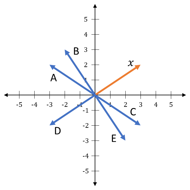
Let \(M = \begin{bmatrix} 1 & 0 \\ 0 & -1 \end{bmatrix}\), and let \(x\) be a 2-element vector as shown. Which vector represents \(M \cdot x\)?

Q7
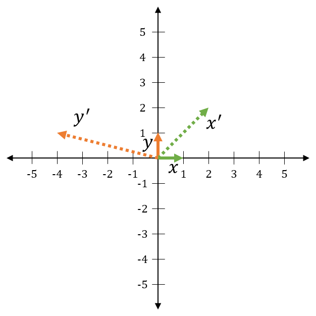
Let \(x = \begin{bmatrix} 1 \\ 0 \end{bmatrix}, \: y = \begin{bmatrix} 0 \\ 1 \end{bmatrix}, \: x' = \begin{bmatrix} 2 \\ 2 \end{bmatrix}, \: y' = \begin{bmatrix} -4 \\ 1 \end{bmatrix}\). Let \(A\) be the matrix that satisfies \(Ax = x'\) and \(Ay = y'\). What is \(A\)?
