Resource Estimation and Practicality Assessment
By now, it's probably becoming clear that the quantum computers we generally have access to today aren't highly capable devices. They only have a handful of qubits, and those qubits are quite prone to quantum errors which make measuring the ideal states unreliable. There are some other, more powerful machines but they aren't open to the general public - you have to have special access in order to use them.
Luckily, not being able to run a circuit on a quantum computer doesn't mean we can't study a circuit's performance. In this section, we're going to talk about how to study the quantum assembly code generated by Qiskit's compiler to glean some insightful information about it's resource requirements and its practicality.
Note
The code below is from the resource_estimate.py file.
You may follow along in that file, execute it, and modify it as you see fit!
Depth, Width, and Gate Count
Let's start with this original circuit:
The Original Circuit (original)
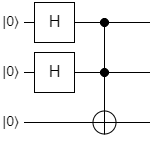
While this is a fairly trivial circuit, it will serve as a good point of comparison for later work.
Let's start by building the circuit:
from qiskit import QuantumCircuit, ClassicalRegister, QuantumRegister
from qiskit.providers.aer import AerSimulator
from qiskit import IBMQ
from qiskit.compiler import transpile
from time import perf_counter

# Initialization
qubits = QuantumRegister(3)
measurement = ClassicalRegister(3)
circuit = QuantumCircuit(qubits, measurement)

# Build the circuit
start = perf_counter()
circuit.h(qubits[0])
circuit.h(qubits[1])
circuit.ccx(qubits[0], qubits[1], qubits[2])
circuit.measure(qubits, measurement)
end = perf_counter()
print(f"Circuit construction took {(end - start)} sec.")
print(circuit)
This will describe how long it took to build the original circuit, thanks to the perf_counter() function.
It will also print it for posterity.
The output will look like this:
Circuit construction took 0.00013719999999994847 sec.
      ┌───┐     ┌─┐
q0_0: ┤ H ├──■──┤M├──────
      ├───┤  │  └╥┘┌─┐
q0_1: ┤ H ├──■───╫─┤M├───
      └───┘┌─┴─┐ ║ └╥┘┌─┐
q0_2: ─────┤ X ├─╫──╫─┤M├
           └───┘ ║  ║ └╥┘
c0: 3/═══════════╩══╩══╩═
                 0  1  2
Next, let's determine the width of the circuit. The width is the total number of qubits required:
# Get the number of qubits needed to run the circuit
active_qubits = {}
for op in circuit.data:
    if op[0].name != "barrier" and op[0].name != "snapshot":
        for qubit in op[1]:
                active_qubits[qubit.index] = True
print(f"Width: {len(active_qubits)} qubits")
This will walk through each gate in the circuit and check which qubits it uses. It will flag all of those qubits as "active", and then tally up the number of active qubits. The output of this code should look like this:
Width: 3 qubits
Note
While Qiskit does provide a QuantumCircuit.width() method, it doesn't actually calculate this value.
It simply sums the sizes of all of the registers involved (both quantum and classical), which can include qubits that don't do anything in the program.
Next, let's get the depth of the circuit. This is the length of the critical path, which is the qubit with the longest irreducible sequence of gates. In the circuit diagram, this is generally the same as the qubit whose gates extend the furthest to the right. Essentially, the depth tells you approximately how long the circuit will be (in terms of number of gates).
Qiskit provides a function that calculates the depth itself quite well via the QuantumCircuit.depth() method:
print(f"Depth: {circuit.depth()}")
Which will output:
Depth: 3
While this number itself isn't enough to gauge how badly an algorithm will be affected by quantum error on a machine, it provides a good ballpark to start analysis with (and provides a good number to compare various implementations of the circuit against).
Finally, let's look at the raw breakdown of gates involved:
print(f"Gate counts: {circuit.count_ops()}")
This will tally up all of the quantum gates in the circuit.
It can be useful when, for example, the CNOT gate is much more error-prone than other gates so you want to come up with an implementation that minimizes the number of CNOT gates at all costs.
The output will look like this:
Gate counts: OrderedDict([('measure', 3), ('h', 2), ('ccx', 1)])
That will be enough to start with.
Transpiling the Circuit
As you know, this circuit will run fine on a simulator but it won't work on a real machine like the ibmq_santiago computer.
We circumvented that during circuit execution by changing the backend parameter.
Here, we're going to dig a bit into that process to actually retrieve the circuit that Qiskit put together to run on that machine without needing to actually run it.
This way, we can get the same metrics you saw above for the modified circuit.
The process of converting one circuit into another one (like what Qiskit does to make the circuit compatible with the machine) is called transpiling.
Let's have Qiskit transpile our circuit above so it can run on santiago:
# Transpile the circuit to something that can run on the Santiago machine
provider = IBMQ.load_account()
machine = "ibmq_santiago"
backend = provider.get_backend(machine)

print(f"Transpiling for {machine}...")
start = perf_counter()
circuit = transpile(circuit, backend=backend, optimization_level=1)
end = perf_counter()
print(f"Compiling and optimizing took {(end - start)} sec.")
print(circuit)
Here the transpile() method from the qiskit.compiler module is the one we need.
If you actually look at its signature, it comes with a lot of parameters you can adjust:
def transpile(circuits: Union[QuantumCircuit, List[QuantumCircuit]],
              backend: Optional[Union[Backend, BaseBackend]] = None,
              basis_gates: Optional[List[str]] = None,
              coupling_map: Optional[Union[CouplingMap, List[List[int]]]] = None,
              backend_properties: Optional[BackendProperties] = None,
              initial_layout: Optional[Union[Layout, Dict, List]] = None,
              layout_method: Optional[str] = None,
              routing_method: Optional[str] = None,
              translation_method: Optional[str] = None,
              scheduling_method: Optional[str] = None,
              instruction_durations: Optional[InstructionDurationsType] = None,
              dt: Optional[float] = None,
              approximation_degree: Optional[float] = None,
              seed_transpiler: Optional[int] = None,
              optimization_level: Optional[int] = None,
              pass_manager: Optional[PassManager] = None,
              callback: Optional[Callable[[BasePass, DAGCircuit, float,
                                           PropertySet, int], Any]] = None,
              output_name: Optional[Union[str, List[str]]] = None) -> Union[QuantumCircuit,
                                                                            List[QuantumCircuit]]:
As you get more and more involved with circuit analysis, you may begin to customize some of these more regularly. For now though, we only care about two things:
- The
backend(you can change this to whatever machine you want, or make a custom object that represents a machine the Qiskit provider can't give you) - The
optimization_level, which describes how hard Qiskit will work to optimize your circuit
With regards to the optimization_level, there are 4 settings:
"""
optimization_level: How much optimization to perform on the circuits.
    Higher levels generate more optimized circuits,
    at the expense of longer transpilation time.
    * 0: no optimization
    * 1: light optimization
    * 2: heavy optimization
    * 3: even heavier optimization
    If ``None``, level 1 will be chosen as default.
"""
You can play around with this if you like - we'll stick to 1 for this walkthrough.
Note
Qiskit's optimizer is still a work in progress; it has some notable difficulties dealing with single-qubit gates as described in this pull request. Keep an eye on this space to see how it improves over time.
With that explanation out of the way, here's the output of the earlier excerpt:
Transpiling for ibmq_santiago...
Compiling and optimizing took 0.9869398 sec.
global phase: π/8
               ┌─────────┐┌────┐┌─────────┐                 ┌───┐                                         ┌─────────┐           ┌───┐     ┌──────────┐   ┌────┐   ┌─────────┐ ░       ┌─┐
     q0_0 -> 0 ┤ RZ(π/2) ├┤ √X ├┤ RZ(π/2) ├──────────■──────┤ X ├──■───────────────────────────────────■──┤ RZ(π/4) ├────────■──┤ X ├──■──┤ RZ(3π/4) ├───┤ √X ├───┤ RZ(π/2) ├─░───────┤M├
               ├─────────┤├────┤├─────────┤        ┌─┴─┐    └─┬─┘┌─┴─┐                     ┌───┐     ┌─┴─┐├─────────┴┐┌───┐┌─┴─┐└─┬─┘┌─┴─┐└──┬───┬───┘┌──┴────┴──┐└──┬───┬──┘ ░    ┌─┐└╥┘
     q0_1 -> 1 ┤ RZ(π/2) ├┤ √X ├┤ RZ(π/2) ├──■─────┤ X ├──────■──┤ X ├──■───────────────■──┤ X ├──■──┤ X ├┤ RZ(7π/4) ├┤ X ├┤ X ├──■──┤ X ├───┤ X ├────┤ RZ(7π/4) ├───┤ X ├────░────┤M├─╫─
               ├─────────┤├────┤├─────────┤┌─┴─┐┌──┴───┴───┐     └───┘┌─┴─┐┌─────────┐┌─┴─┐└─┬─┘┌─┴─┐└───┘└──────────┘└─┬─┘└───┘     └───┘   └─┬─┘    ├─────────┬┘   └─┬─┘    ░ ┌─┐└╥┘ ║
     q0_2 -> 2 ┤ RZ(π/2) ├┤ √X ├┤ RZ(π/2) ├┤ X ├┤ RZ(7π/4) ├──────────┤ X ├┤ RZ(π/4) ├┤ X ├──■──┤ X ├───────────────────■──────────────────────■──────┤ RZ(π/4) ├──────■──────░─┤M├─╫──╫─
               └─────────┘└────┘└─────────┘└───┘└──────────┘          └───┘└─────────┘└───┘     └───┘                                                 └─────────┘             ░ └╥┘ ║  ║
ancilla_0 -> 3 ───────────────────────────────────────────────────────────────────────────────────────────────────────────────────────────────────────────────────────────────░──╫──╫──╫─
                                                                                                                                                                              ░  ║  ║  ║
ancilla_1 -> 4 ───────────────────────────────────────────────────────────────────────────────────────────────────────────────────────────────────────────────────────────────░──╫──╫──╫─
                                                                                                                                                                              ░  ║  ║  ║
         c0: 3/══════════════════════════════════════════════════════════════════════════════════════════════════════════════════════════════════════════════════════════════════╩══╩══╩═
                                                                                                                                                                                 0  1  2
  active_qubits[qubit.index] = True
Width: 3 qubits
Depth: 22
Gate counts: OrderedDict([('cx', 15), ('rz', 14), ('sx', 4), ('measure', 3), ('barrier', 1)])
As a reminder, both of these circuits do the same thing.
The difference is that this circuit is made of gates that the ibmq_santiago machine supports and respects its qubit connectivity map, where not all qubits can interact with each other directly.
It still has a width of 3 qubits, which means it is able to run on that machine (since the machine has 5 qubits), but the depth increased from 3 to 22.
It also has 15 CNOT gates, whereas the original circuit only had 1 CCNOT gate.
This will certainly have implications when it comes to how long the circuit takes to run and how many errors it will encounter.
Needless to say, this circuit is substantially more complicated than the original, but the hardware cannot run the original. Thus, in order to study if a quantum algorithm is actually runnable on a given quantum computer, you need to do this kind of assessment. Observing the general figures from a research paper won't be enough.
Estimating Runtime
Accurately approximating how long a circuit will take to execute is a bit of a challenge. To do it, you need to know the entire gate sequence in the critical path and how long each of those gates takes to execute.
For the critical path gate sequence, you'll have to manually find this. You can do it by modifying the code used to get the circuit depth; you'll want to keep track of the gates and qubits involved in each path, rather than just the length of the path itself.
For gat eexecution time, IBM makes this information available for its own systems within the backend object.
You can get the raw gate information from like this:
backend.properties().gates
Each gate on each qubit (or combination of qubits in the case of cx) has its own entry in this list.
You can retrieve information about this gate like so (for example, on the first gate in the list):
backend.properties().gates[0].to_dict()
The output will be something similar to this:
{
  "qubits": [ 0 ],
  "gate": "id",
  "parameters": [
    {
      "date": "datetime.datetime(2021, 6, 29, 0, 21, 42, tzinfo=tzlocal())",
      "name": "gate_error",
      "unit": "",
      "value": 0.0001881646337499316
    },
    {
      "date": "datetime.datetime(2021, 6, 29, 11, 52, 26, tzinfo=tzlocal())",
      "name": "gate_length",
      "unit": "ns",
      "value": 35.55555555555556
    }
  ],
  "name": "id0"
}
This tells you what gate it is (the id gate here), what qubits it applies to (qubit 0), what its error rate is (0.01881% chance of error), and how long it takes to run (35.56 nanoseconds).
You'll need to cross-reference the gates and qubits from the critical path with this list to determine the length of the critical path.
Simulating Noise to Assess Practicality
When it comes to assessing error rates for an overall circuit, it can become difficult to model the probabilities of each gate causing an error, and then the subsequent effects that will have on the rest of the circuit. Luckily, Qiskit lets you embed all of the details for a quantum machine (e.g. its connectivity map, its native gates, and their individual error rates) into its simulator. This means you can run a circuit on the simulator using the timing and error profile of the real machine, without needing the real machine.
Here's how you do it:
# Simulate a run on Santiago, using its real gate information to model the output with real errors
santiago_sim = AerSimulator.from_backend(backend)
result = santiago_sim.run(circuit).result()
counts = result.get_counts(circuit)
for(measured_state, count) in counts.items():
    big_endian_state = measured_state[::-1]
    print(f"Measured {big_endian_state} {count} times.")
The key here is the AerSimulator.from_backend() method.
If you already have a backend object with all of your machine's physical characteristics described, you can just pass that into Qiskit's simulator and it will take care of the rest.
You just have to run the circuit using the run() method instead of the execute() method.
Once this executes, you'll see the following output:
Measured 000 252 times.
Measured 100 229 times.
Measured 111 230 times.
Measured 010 232 times.
Measured 110 32 times.
Measured 001 18 times.
Measured 101 16 times.
Measured 011 15 times.
This is very similar to the real output we got on the real machine in the previous section. Nice!
The main benefit of this technique is that it lets you "simulate" a real machine is it's not available (the queue is too long, it's down for maintenance, or you simply don't have access to it). In the latter case, you can either create your own backend, or use IBM's massive repository of "mock" backends. Each one of these has all of the gate and connectivity information for its real systems (including ones you don't have access to, such as the 27-qubit Montreal machine).
To use them, all you need is to import the appropriate device from the qiskit.test.mock module.
For example, here's how to load the Montreal-based test backend:
from qiskit.test.mock import FakeMontreal
montreal_backend = FakeMontreal()
Now, you can use montreal_backend anywhere you'd use a normal backend, such as the transpile() method for circuit generation or the AerSimulator.from_backend() method to create a simulator with Montreal as its execution and noise model.
If we run our above circuit through the transpiler and simulator process, here's what we get:
Transpiling for ibmq_montreal...
Compiling and optimizing took 0.0817944000000006 sec.
global phase: π/8
                 ┌─────────┐┌────┐┌─────────┐                                                                                                 ┌─────────┐             ░ ┌─┐
       q0_0 -> 0 ┤ RZ(π/2) ├┤ √X ├┤ RZ(π/2) ├──────────────────────────────────■────────────────────────────────■──────────────────────■──────┤ RZ(π/4) ├──────■──────░─┤M├──────
                 ├─────────┤├────┤├─────────┤                      ┌───┐     ┌─┴─┐┌─────────┐┌───┐┌──────────┐┌─┴─┐     ┌───┐        ┌─┴─┐    ├─────────┴┐   ┌─┴─┐    ░ └╥┘┌─┐
       q0_1 -> 1 ┤ RZ(π/2) ├┤ √X ├┤ RZ(π/2) ├──■────────────────■──┤ X ├──■──┤ X ├┤ RZ(π/4) ├┤ X ├┤ RZ(7π/4) ├┤ X ├──■──┤ X ├──■─────┤ X ├────┤ RZ(7π/4) ├───┤ X ├────░──╫─┤M├───
                 ├─────────┤├────┤├─────────┤┌─┴─┐┌──────────┐┌─┴─┐└─┬─┘┌─┴─┐└───┘└─────────┘└─┬─┘├─────────┬┘└───┘┌─┴─┐└─┬─┘┌─┴─┐┌──┴───┴───┐└──┬────┬──┘┌──┴───┴──┐ ░  ║ └╥┘┌─┐
       q0_2 -> 2 ┤ RZ(π/2) ├┤ √X ├┤ RZ(π/2) ├┤ X ├┤ RZ(7π/4) ├┤ X ├──■──┤ X ├──────────────────■──┤ RZ(π/4) ├──────┤ X ├──■──┤ X ├┤ RZ(3π/4) ├───┤ √X ├───┤ RZ(π/2) ├─░──╫──╫─┤M├
                 └─────────┘└────┘└─────────┘└───┘└──────────┘└───┘     └───┘                     └─────────┘      └───┘     └───┘└──────────┘   └────┘   └─────────┘ ░  ║  ║ └╥┘
  ancilla_0 -> 3 ─────────────────────────────────────────────────────────────────────────────────────────────────────────────────────────────────────────────────────░──╫──╫──╫─
                                                                                                                                                                      ░  ║  ║  ║
  ancilla_1 -> 4 ─────────────────────────────────────────────────────────────────────────────────────────────────────────────────────────────────────────────────────░──╫──╫──╫─
                                                                                                                                                                      ░  ║  ║  ║
  ancilla_2 -> 5 ─────────────────────────────────────────────────────────────────────────────────────────────────────────────────────────────────────────────────────░──╫──╫──╫─
                                                                                                                                                                      ░  ║  ║  ║
  ancilla_3 -> 6 ─────────────────────────────────────────────────────────────────────────────────────────────────────────────────────────────────────────────────────░──╫──╫──╫─
                                                                                                                                                                      ░  ║  ║  ║
  ancilla_4 -> 7 ─────────────────────────────────────────────────────────────────────────────────────────────────────────────────────────────────────────────────────░──╫──╫──╫─
                                                                                                                                                                      ░  ║  ║  ║
  ancilla_5 -> 8 ─────────────────────────────────────────────────────────────────────────────────────────────────────────────────────────────────────────────────────░──╫──╫──╫─
                                                                                                                                                                      ░  ║  ║  ║
  ancilla_6 -> 9 ─────────────────────────────────────────────────────────────────────────────────────────────────────────────────────────────────────────────────────░──╫──╫──╫─
                                                                                                                                                                      ░  ║  ║  ║
 ancilla_7 -> 10 ─────────────────────────────────────────────────────────────────────────────────────────────────────────────────────────────────────────────────────░──╫──╫──╫─
                                                                                                                                                                      ░  ║  ║  ║
 ancilla_8 -> 11 ─────────────────────────────────────────────────────────────────────────────────────────────────────────────────────────────────────────────────────░──╫──╫──╫─
                                                                                                                                                                      ░  ║  ║  ║
 ancilla_9 -> 12 ─────────────────────────────────────────────────────────────────────────────────────────────────────────────────────────────────────────────────────░──╫──╫──╫─
                                                                                                                                                                      ░  ║  ║  ║
ancilla_10 -> 13 ─────────────────────────────────────────────────────────────────────────────────────────────────────────────────────────────────────────────────────░──╫──╫──╫─
                                                                                                                                                                      ░  ║  ║  ║
ancilla_11 -> 14 ─────────────────────────────────────────────────────────────────────────────────────────────────────────────────────────────────────────────────────░──╫──╫──╫─
                                                                                                                                                                      ░  ║  ║  ║
ancilla_12 -> 15 ─────────────────────────────────────────────────────────────────────────────────────────────────────────────────────────────────────────────────────░──╫──╫──╫─
                                                                                                                                                                      ░  ║  ║  ║
ancilla_13 -> 16 ─────────────────────────────────────────────────────────────────────────────────────────────────────────────────────────────────────────────────────░──╫──╫──╫─
                                                                                                                                                                      ░  ║  ║  ║
ancilla_14 -> 17 ─────────────────────────────────────────────────────────────────────────────────────────────────────────────────────────────────────────────────────░──╫──╫──╫─
                                                                                                                                                                      ░  ║  ║  ║
ancilla_15 -> 18 ─────────────────────────────────────────────────────────────────────────────────────────────────────────────────────────────────────────────────────░──╫──╫──╫─
                                                                                                                                                                      ░  ║  ║  ║
ancilla_16 -> 19 ─────────────────────────────────────────────────────────────────────────────────────────────────────────────────────────────────────────────────────░──╫──╫──╫─
                                                                                                                                                                      ░  ║  ║  ║
ancilla_17 -> 20 ─────────────────────────────────────────────────────────────────────────────────────────────────────────────────────────────────────────────────────░──╫──╫──╫─
                                                                                                                                                                      ░  ║  ║  ║
ancilla_18 -> 21 ─────────────────────────────────────────────────────────────────────────────────────────────────────────────────────────────────────────────────────░──╫──╫──╫─
                                                                                                                                                                      ░  ║  ║  ║
ancilla_19 -> 22 ─────────────────────────────────────────────────────────────────────────────────────────────────────────────────────────────────────────────────────░──╫──╫──╫─
                                                                                                                                                                      ░  ║  ║  ║
ancilla_20 -> 23 ─────────────────────────────────────────────────────────────────────────────────────────────────────────────────────────────────────────────────────░──╫──╫──╫─
                                                                                                                                                                      ░  ║  ║  ║
ancilla_21 -> 24 ─────────────────────────────────────────────────────────────────────────────────────────────────────────────────────────────────────────────────────░──╫──╫──╫─
                                                                                                                                                                      ░  ║  ║  ║
ancilla_22 -> 25 ─────────────────────────────────────────────────────────────────────────────────────────────────────────────────────────────────────────────────────░──╫──╫──╫─
                                                                                                                                                                      ░  ║  ║  ║
ancilla_23 -> 26 ─────────────────────────────────────────────────────────────────────────────────────────────────────────────────────────────────────────────────────░──╫──╫──╫─
                                                                                                                                                                      ░  ║  ║  ║
           c0: 3/════════════════════════════════════════════════════════════════════════════════════════════════════════════════════════════════════════════════════════╩══╩══╩═
                                                                                                                                                                         0  1  2
Width: 3 qubits
Depth: 20
Gate counts: OrderedDict([('rz', 14), ('cx', 12), ('sx', 4), ('measure', 3), ('barrier', 1)])
Measured 001 13 times.
Measured 111 208 times.
Measured 100 234 times.
Measured 010 226 times.
Measured 101 30 times.
Measured 000 260 times.
Measured 110 19 times.
Measured 011 34 times.
As you can see, the fact that the machine has more qubits doesn't make much of a difference for our circuit. All but 3 of them are idle, and the error rate appears to be the same which is expected, since the qubits and gates themselves have the same physical implementation as the Santiago machine. The depth is 20 instead of 22, and the circuit itself looks a bit different, but from a practical perspective the measurements appear to be about the same.
Drawing Conclusions
The tools and techniques shown here are excellent for taking a quantum algorithm, implementing it in code, and then studying what that algorithm looks like when built for real quantum computers. While the high-level theory of the algorithm typically offers some complexity analysis that gives you a general view of how efficient an algorithm is and how many qubits it takes, you can't really know these details until you build the quantum assembly and try it out for real.
Using this knowledge, you will be able to definitely tell if a quantum computer has enough qubits to support your algorithm, study various different implementations of the circuit to find the shortest (or perhaps the least error-prone) version, and describe what the end measurements will look like. If they're sufficiently scrambled and the "correct" answer is lost in the noise, then you can clearly see that using Qiskit's real execution or simulation engine.
Being able to study an algorithm in this way is a very useful skill to have - especially as quantum computing grows in popularity.